 |
Each data mining algorithm generated its own rule set to evaluate new examples. These detection models were the final result of our experiments. Each algorithm's rule set could be incorporated into a scanner to detect malicious programs. The generation of the rules only needed to be done periodically and the rule set distributed in order to detect new malicious executables.
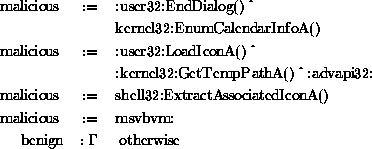
RIPPER's rules were built to generalize over unseen examples so the rule set was more compact than the signature based methods. For the data set that contained 3,301 malicious executables the RIPPER rule set contained the five rules in Figure 5.
Here, a malicious executable was consistent with one of four hypotheses:
A binary is labeled benign if it is inconsistent with all of the malicious binary hypotheses in Figure 5.
The Naive Bayes rules were more complicated than the RIPPER and signature based hypotheses. These rules took the form of P(F|C), the probability of an example F given a class C. The probability for a string occurring in a class is the total number of times it occurred in that class's training set divided by the total number of times that the string occurred over the entire training set. These hypotheses are illustrated in Figure 6.
Here, the string ``windows'' was predicted to more likely to occur in a benign program and string ``*.COM'' was more than likely in a malicious executable program.
However this leads to a problem when a string (e.g. ``CH2OH-CHOH-CH2OH'') only occurred in one set, for example only in the malicious executables. The probability of ``CH20H-CHOH-CH20H'' occurring in any future benign example is predicted to be 0, but this is an incorrect assumption. If a Chemistry TA's program was written to print out ``CH20H-CHOH-CH20H'' (glycerol) it will always be tagged a malicious executable even if it has other strings in it that would have labeled it benign.
In Figure 6 the string ``*.COM" does not occur in any benign programs so the probability of ``*.COM" occurring in class benign is approximated to be 1/12 instead of 0/11. This approximates real world probability that any string could occur in both classes even if during training it was only seen in one class [9].
The rule sets generated by our Multi-Naive Bayes algorithm are the collection of the rules generated by each of the component Naive Bayes classifiers. For each classifier, there is a rule set such as the one in Figure 6. The probabilities in the rules for the different classifiers may be different because the underlying data that each classifier is trained on is different. The prediction of the Multi-Naive Bayes algorithm is the product of the predictions of the underlying Naive Bayes classifiers.